Making sense out of tracker orientation data

Here we describe what we did to make sense out of the orientation data from our Polhemus Liberty tracking device. Maybe this is useful for someone…

First, we tried to find the tracker coordinate system in the real world. For this test we printed the position data to stdout and did two steps:

• tried to find the origin.

• tried to find the x-, y- and z-axis by moving in the directions where the respective values become bigger (this coordinate system is also marked on the emitter box).

After that we knew the global coordinate frame, so we could tackle the orientation of the markers.

For the orientation tests we needed to record the data and display an animation.

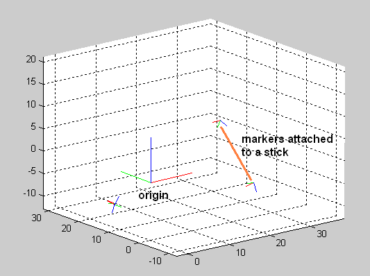
We converted the measured data to a rotation matrix. Then we displayed small coordinate systems at the marker positions using the columns of that matrix.

We computed the rotation matrices that rotate 45 degrees around the x- y- and z-axis and displayed them together with the global reference coordinate system. We checked if this is valid!

We needed these coordinate frames to display an animation of the recorded data. Also, it was also a good idea to draw the global reference and a grid.

We attached (at least) two markers rigidly to a stick or board. they must not move with repect to each other.

1. We moved the board (without rotating it) in the direction +x and back. We did the same in y and z-direction. (This gave us confidence that we got the position right)
2. We turned the object with both sensors attached around the x-axis in positive direction. We did the same with the y- an z-axis. (Now we had two markers for which we knew and saw how they must turn)

Now, that we had the test data, we replayed the animation:

First, we checked whether the board moves in the correct directions. That was the case, so we knew that our position data is correct. If not, we would have fixed this error first.

If the orientation is also correct, the marker coordinate frames rotate as if they are rigidly attached to each other.

If the coordinate systems rotate in opposite directions, chances are, that we must transpose our rotation matrix.

That was not the case, so we checked the angle conversion function:

They essentially consist of the axis of rotation and the cosine of the angle (and all that normalized to length 1) There are two different versions around, one which specifies the angle first and then the axis. The other is vice versa. So, if our quaternion is q = [q1, q2, q3, q4] we try also [q2, q3, q4, q1] and [q4, q1, q2, q3]. Just in case ;)

The formula is:

% q = [q0 qx qy qz]

m = [[(q(1)*q(1) + q(2)*q(2) - q(3)*q(3) - q(4)*q(4)), ...
    2*(q(2)*q(3) - q(1)*q(4)), ...
    2*(q(2)*q(4) + q(1)*q(3))]; ...
   [2*(q(3)*q(2) + q(1)*q(4)), ...
    (q(1)*q(1) - q(2)*q(2) + q(3)*q(3) - q(4)*q(4)), ...
    2*(q(3)*q(4) - q(1)*q(2))]; ...
   [2*(q(4)*q(2) - q(1)*q(3)), ...
    2*(q(4)*q(3) + q(1)*q(2)), ...
    (q(1)*q(1) - q(2)*q(2) - q(3)*q(3) + q(4)*q(4))]];

There are a number of different ways to calculate the matrix here. It is always a product of three rotation matrices. We also tried negating the angles.

Fortunately this was very verbosely described in the manual. In our case the formula was:

m = rotx(roll)*roty(elevation)*rotz(azimuth);

This means: first rotate around the z-axis with angle azimuth, then rotate around the y-axis with angle elevation and lastly rotate around the x-axis with angle roll. The rightmost rotation is carried out first!

The implementation of this animation viewer was done in Matlab and is now part of a joint calibration method which is described here.